stanで求めたMCMCサンプルからサベージ・ディッキー法でベイズファクターを計算してみた.
使用は自己責任で….
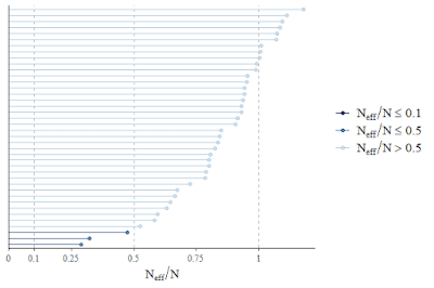
Neff/N
Rhat

box plot

使用は自己責任で….
> # load package
> library(rstan) # mcmcを実行するstanをrで動かすパッケージ
 要求されたパッケージ StanHeaders をロード中です
rstan (Version 2.19.2, GitRev: 2e1f913d3ca3)
For execution on a local, multicore CPU with excess RAM we recommend calling
options(mc.cores = parallel::detectCores()).
To avoid recompilation of unchanged Stan programs, we recommend calling
rstan_options(auto_write = TRUE)
For improved execution time, we recommend calling
Sys.setenv(LOCAL_CPPFLAGS = '-march=native')
although this causes Stan to throw an error on a few processors.
Warning messages:
1:  パッケージ ‘rstan’ はバージョン 3.6.1 の R の下で造られました
2:  パッケージ ‘StanHeaders’ はバージョン 3.6.1 の R の下で造られました
> library(rstanarm)  # stanのラップパッケージで,これでベイジアン階層モデルを簡単に使える
> library(afex) # 今回のテストデータのために読み込むパッケージ,本当はこのパッケージでMANOVA,MixedModel等色々できる
 要求されたパッケージ lme4 をロード中です
 要求されたパッケージ Matrix をロード中です

 次のパッケージを付け加えます: ‘lme4’

 以下のオブジェクトは ‘package:brms’ からマスクされています:

     ngrps

Registered S3 methods overwritten by 'car':
  method                          from
  influence.merMod                lme4
  cooks.distance.influence.merMod lme4
  dfbeta.influence.merMod         lme4
  dfbetas.influence.merMod        lme4
************
Welcome to afex. For support visit: http://afex.singmann.science/
- Functions for ANOVAs: aov_car(), aov_ez(), and aov_4()
- Methods for calculating p-values with mixed(): 'KR', 'S', 'LRT', and 'PB'
- 'afex_aov' and 'mixed' objects can be passed to emmeans() for follow-up tests
- NEWS: library('emmeans') now needs to be called explicitly!
- Get and set global package options with: afex_options()
- Set orthogonal sum-to-zero contrasts globally: set_sum_contrasts()
- For example analyses see: browseVignettes("afex")
************

 次のパッケージを付け加えます: ‘afex’

 以下のオブジェクトは ‘package:lme4’ からマスクされています:

     lmer

> # data preparation
> data("md_12.1")
> head(md_12.1)
  id  noise angle  rt
1  1 absent     0 420
2  2 absent     0 420
3  3 absent     0 480
4  4 absent     0 420
5  5 absent     0 540
6  6 absent     0 360
> summary(md_12.1) # rt 以外は全てfactorであることに注意
       id         noise    angle        rt
 1      : 6   absent :30   0:20   Min.   :360
 2      : 6   present:30   4:20   1st Qu.:480
 3      : 6                8:20   Median :540
 4      : 6                       Mean   :569
 5      : 6                       3rd Qu.:660
 6      : 6                       Max.   :900
 (Other):24
> # model building
> fit<- stan_lmer(
+   formula = rt ~ angle + (1 + angle |id),       #式 lme4とほぼ同じ,,今回は被験者にランダム切片とランダム傾き
+   data = md_12.1,                               #データ名
+   )

SAMPLING FOR MODEL 'continuous' NOW (CHAIN 1).
Chain 1:
Chain 1: Gradient evaluation took 0 seconds
Chain 1: 1000 transitions using 10 leapfrog steps per transition would take 0 seconds.
Chain 1: Adjust your expectations accordingly!
Chain 1:
Chain 1:
Chain 1: Iteration:    1 / 2000 [  0%]  (Warmup)
Chain 1: Iteration:  200 / 2000 [ 10%]  (Warmup)

# 一部省略

Chain 4: Iteration:  800 / 2000 [ 40%]  (Warmup)
Chain 4: Iteration: 1000 / 2000 [ 50%]  (Warmup)
Chain 4: Iteration: 1001 / 2000 [ 50%]  (Sampling)
Chain 4: Iteration: 1200 / 2000 [ 60%]  (Sampling)
Chain 4: Iteration: 1400 / 2000 [ 70%]  (Sampling)
Chain 4: Iteration: 1600 / 2000 [ 80%]  (Sampling)
Chain 4: Iteration: 1800 / 2000 [ 90%]  (Sampling)
Chain 4: Iteration: 2000 / 2000 [100%]  (Sampling)
Chain 4:
Chain 4:  Elapsed Time: 5.017 seconds (Warm-up)
Chain 4:                2.622 seconds (Sampling)
Chain 4:                7.639 seconds (Total)
Chain 4:

> fit
stan_lmer
 family:       gaussian [identity]
 formula:      rt ~ angle + (1 + angle | id)
 observations: 60
------
            Median MAD_SD
(Intercept) 478.3   28.5
angle4      105.7   37.6
angle8      166.6   38.1

Auxiliary parameter(s):
      Median MAD_SD
sigma 111.5   11.9

Error terms:
 Groups   Name        Std.Dev. Corr
 id       (Intercept)  48
          angle4       35      0.03
          angle8       39      0.08 0.23
 Residual             112
Num. levels: id 10

Sample avg. posterior predictive distribution of y:
         Median MAD_SD
mean_PPD 569.0   20.2

------
* For help interpreting the printed output see ?print.stanreg
* For info on the priors used see ?prior_summary.stanreg
> # model estimaion
> library(bayesplot)
This is bayesplot version 1.7.0
- Online documentation and vignettes at mc-stan.org/bayesplot
- bayesplot theme set to bayesplot::theme_default()
   * Does _not_ affect other ggplot2 plots
   * See ?bayesplot_theme_set for details on theme setting
> mcmc_neff(neff_ratio(fit)) #0.1以上
> mcmc_rhat(rhat(fit)) #1.1未満
> # effect calculation
> library(emmeans)
> effect<-emmeans(fit, ~ angle) #周辺化平均でメインエフェクトをみる
> effect
 angle emmean lower.HPD upper.HPD
 0        478       423       536
 4        585       523       649
 8        644       575       706

HPD interval probability: 0.95
> diff_eff<-pairs(effect) #bayesfactor計算のためペアの差を抜き出し
> diff_eff
 contrast estimate lower.HPD upper.HPD
 0 - 4      -105.7      -178     -33.7
 0 - 8      -166.6      -237     -89.4
 4 - 8       -60.7      -143      13.9

HPD interval probability: 0.95
> # bayes factor
> library(bayestestR)
> bayesfactor_savagedickey(diff_eff, prior = fit)
Computation of Bayes factors: sampling priors, please wait...
# Bayes Factor (Savage-Dickey density ratio)

 Parameter Bayes Factor
     0 - 4         5.09
     0 - 8       107.84
     4 - 8          0.3
---
Evidence Against Test Value:  0

# graphic
> library(tidybayes)

 次のパッケージを付け加えます: ‘tidybayes’

 以下のオブジェクトは ‘package:bayestestR’ からマスクされています:

     hdi

> ext_effect<-gather_emmeans_draws(effect) #描画のためメインエフェクトの取り出し
> summary(ext_effect) #.valueが値です
 angle        .chain        .iteration        .draw          .value
 0:4000   Min.   : NA     Min.   : NA     Min.   :   1   Min.   :377.1
 4:4000   1st Qu.: NA     1st Qu.: NA     1st Qu.:1001   1st Qu.:496.3
 8:4000   Median : NA     Median : NA     Median :2000   Median :582.1
          Mean   :NaN     Mean   :NaN     Mean   :2000   Mean   :568.6
          3rd Qu.: NA     3rd Qu.: NA     3rd Qu.:3000   3rd Qu.:629.4
          Max.   : NA     Max.   : NA     Max.   :4000   Max.   :792.3
          NA's   :12000   NA's   :12000
> library(ggplot2)
> ggplot(data = ext_effect, aes(x = angle, y = .value)) +
+   geom_boxplot(outlier.colour = NA) +
+   ylim(0,800)
>
Neff/N

Rhat

box plot

コメント